Slave Spins Mean Field Theory
Construction
Start from the observation that the possible occupancies of a real fermion( )
on a given site,
)
on a given site,  and
and  , can be
represented as two possible states of a spin-
, can be
represented as two possible states of a spin- variable,
  and
and
 . The idea then is to duplicate the original particle into a spin-like
degree of freedom and a fermion charge degree of freedom by introducing a spin-field and
an associated auxiliary fermion(
. The idea then is to duplicate the original particle into a spin-like
degree of freedom and a fermion charge degree of freedom by introducing a spin-field and
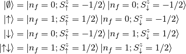
an associated auxiliary fermion( ). In this manner vacuum state and occupied
states are represented as:
). In this manner vacuum state and occupied
states are represented as:
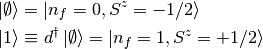
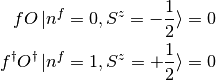
In this context, the anti-commutation properties of the original fermion
operator are insured by the introduction of the auxiliary fermion
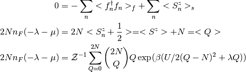
operator . Then, one formulates the constrain:
(1)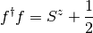
which insures that the number of auxiliary fermions and the spin’s states are the same and, above all, it eliminates the non-physical states
It is important to note that the spin- variable has nothing to do with the
actual spin of the particle. The slave spin- variable is introduced for
every fermion species to give the presence of the particle. Therefore, the
original particle  is replicated into the slave variables with the
same quantum numbers:
is replicated into the slave variables with the
same quantum numbers:  and
and  . To exemplify this, the
orbital base
. To exemplify this, the
orbital base 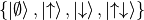 is written in this extended Hilbert space as:
Then when dealing with a multi orbital system,  new spin- variables
 and auxiliary fermions
  are introduced, where
 is the number of orbitals.
Case: The isolated atom
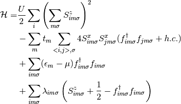
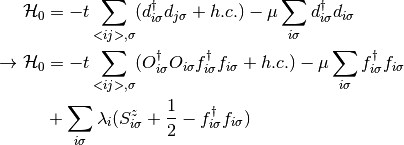
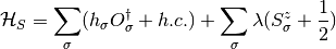
In order to test the slave-spin method, we first consider the case of a degenerate multi-orbital atom, whose analytical solution is well known. The Hamiltonian in particle-hole symmetry formulation reads:
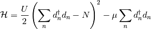
The first step is to recast the Hamiltonian in terms of the new slave-spin
operators. The first choice is to use the auxiliary
fermions for the non-interacting term( ) and the slave spins for the interacting case(
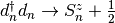 ). We seek a paramagnetic solution, then the constraint
(1) which avoids non-physical states
is included through a unique Lagrange multiplier
). We seek a paramagnetic solution, then the constraint
(1) which avoids non-physical states
is included through a unique Lagrange multiplier  , since all particles
are indistinguishable in spin and orbital quantum numbers. After this treatment
the Hamiltonian reads:
, since all particles
are indistinguishable in spin and orbital quantum numbers. After this treatment
the Hamiltonian reads:
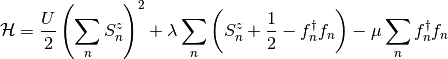
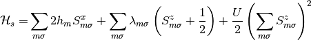
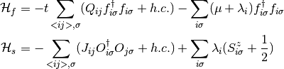
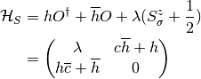
which is possible to separate into a fermion and a spin Hamiltonians:
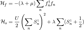
The spin Hamiltonian has a spectrum  ,
where
,
where  is the charge present.The Lagrange multiplier is fixed at the mean-field level by
determining the stationary point of the mean-field averaged Hamiltonian:
is the charge present.The Lagrange multiplier is fixed at the mean-field level by
determining the stationary point of the mean-field averaged Hamiltonian:
 . Within this
approach, the restriction (1) is therefore
respected at the mean field level too.
. Within this
approach, the restriction (1) is therefore
respected at the mean field level too.
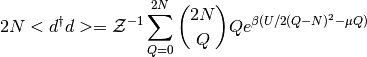
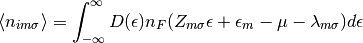
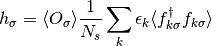
Where every term is averaged with its corresponding Hamiltonian,  is the Fermi
distribution and the Grand Canonical Partition function from the spin
Hamiltonian is
is the Fermi
distribution and the Grand Canonical Partition function from the spin
Hamiltonian is
 .
Then by numerical root finding the
multiplier
.
Then by numerical root finding the
multiplier  can be estimated and allows to describe
the mean fermion occupation,
which is
can be estimated and allows to describe
the mean fermion occupation,
which is 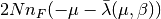 . The
solution that we find can be conveniently represented by the total fermion
occupation as a function of the chemical potential
. The
solution that we find can be conveniently represented by the total fermion
occupation as a function of the chemical potential  . The resulting curve
displays the well known Coulomb ladder-shape,
where the system acquires only integer fillings. The change from an integer
occupation to an adjacent one takes place abruptly as a function of the
chemical potential .
. The resulting curve
displays the well known Coulomb ladder-shape,
where the system acquires only integer fillings. The change from an integer
occupation to an adjacent one takes place abruptly as a function of the
chemical potential .
It is necessary to compare the slave spins solution to the exact solution, given by:
As shown in the next plot, the slave spin approximation is capable of recovering the coulomb occupation ladder, for the isolated atom with degenerate fermions in spin and orbital. The approximation works best around half-filling.
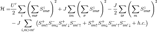
Case: The lattice model - The Hubbard Model
When in a lattice, atoms have overlapping orbitals and electrons are capable to
move along this lattice. Then for the Hamiltonian this term needs to be
included appearing in the Tight-Binding formulation. Then as simple extension
of the previous isolated atom case and in a multi-orbital scenario, the
Hamiltonian reads. The focus now for simplicity is the case of zero crystal-field splitting
 and half-filling of each band one electron per site in each
orbital
and half-filling of each band one electron per site in each
orbital  .
.
(2)
Here it is needed to enforce the restriction:
(3)
using the Lagrange multiplier  , which can be used declaring
specific constrains to lattice site, orbital, and spin.
, which can be used declaring
specific constrains to lattice site, orbital, and spin.
When rewriting the Hamiltonian in terms of the auxiliary fermions and the slave spins the interaction term turns easily into:
For the non interacting part, an appropriate representation of the creation
operator has to be chosen. The direct possibility  ,
although correct leads to problems with the spectral weight conservation because
,
although correct leads to problems with the spectral weight conservation because
 and
and  don’t commute. Instead the representation
  and
and  is chosen, which is identical on the physical Hilbert
space and involves commuting slave spin operators.
is chosen, which is identical on the physical Hilbert
space and involves commuting slave spin operators.
The constrain is treated on average using a static and
site, orbital and particle independent Lagrange multiplier .
Then the Hamiltonian reads:
Using a Hartree-Fock approximation for the operators  and :
and :
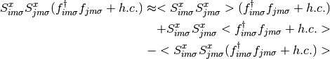
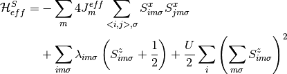
it is then possible to decouple the Hamiltonian into two effective ones:
(4)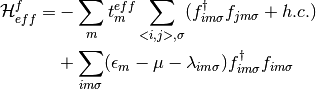
(5)
Where the effective hopping and the effective exchange constants are determined self consistently from:
(6)
(7)
The fermion field Hamiltonian is a non-interacting one, and it’s analytical solution is well known. For the slave spin Hamiltonian, it can be treated in a single-site using the Weiss mean field approximation.
(8)
Here the mean field  has to be determined self-consistently from:
(9)
 is the coordination number,
  with
with  the set of vectors to the nearest neighbours
The effective fermion Hamiltonian is
(10)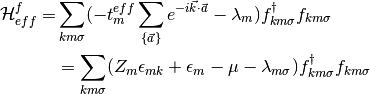
where  is the quasiparticle weight.
In the ordered spin basis  , where the spin labelling the operators are then
![S^z_{\uparrow} = \frac{1}{2} \left[\begin{smallmatrix}1 & 0 & 0 & 0\\0 & 1 & 0 & 0\\0 & 0 & -1 & 0\\0 & 0 & 0 & -1\end{smallmatrix}\right]](_images/math/2cbfb6591552dae0b11c2c4ba1119e939f5b2d0e.png)
![S^z_{\downarrow} = \frac{1}{2} \left[\begin{smallmatrix}1 & 0 & 0 & 0\\0 & -1 & 0 & 0\\0 & 0 & 1 & 0\\0 & 0 & 0 & -1\end{smallmatrix}\right]](_images/math/f045b0c2f11cffa9f5db8804b6f7a42f582a6cb8.png)
![S^x_{\uparrow} = \frac{1}{2} \left[\begin{smallmatrix}0 & 0 & 1 & 0\\0 & 0 & 0 & 1\\1 & 0 & 0 & 0\\0 & 1 & 0 & 0\end{smallmatrix}\right]](_images/math/282dbf92a8328ea4edd74073be0ba8010c7862dd.png)
![S^x_{\downarrow} = \frac{1}{2} \left[\begin{smallmatrix}0 & 1 & 0 & 0\\1 & 0 & 0 & 0\\0 & 0 & 0 & 1\\0 & 0 & 1 & 0\end{smallmatrix}\right]](_images/math/ecc8d719414723fe9ee4570e3a3b50137b5c64f3.png)
As seen in equations (2)
there is no hybridization between bands, hopping preserves then the orbital
quantum number.
When treating the system within a local mean field, in absence of hybridization
the  dependence enters the problem only through each band dispersion
as seen in equations (9), (10). Sums
over momenta can thus be replaced by integrals over the energy weighted by the
density of states
dependence enters the problem only through each band dispersion
as seen in equations (9), (10). Sums
over momenta can thus be replaced by integrals over the energy weighted by the
density of states  , which is specific to the
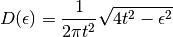
lattice geometry and dimension. For this work, as commonly employed in the
literature, the Bethe lattice will be used. It has a very simple semi-circular
form of the density of states:
, which is specific to the
lattice geometry and dimension. For this work, as commonly employed in the
literature, the Bethe lattice will be used. It has a very simple semi-circular
form of the density of states:
(11)
and allows to simplify calculations in a great amount. Here  is the
hopping amplitude and the half-bandwidth is
is the
hopping amplitude and the half-bandwidth is  , which is set as
the energy unit throughout this work. It is known moreover that the Bethe
lattice
well portrays the salient physical properties of the Mott-Hubbard transition and
it has immediate connection with the dynamical mean field
theory [Georges1996], which is exact in the infinite dimensions limit
and which we intend to implement in future
work.
, which is set as
the energy unit throughout this work. It is known moreover that the Bethe
lattice
well portrays the salient physical properties of the Mott-Hubbard transition and
it has immediate connection with the dynamical mean field
theory [Georges1996], which is exact in the infinite dimensions limit
and which we intend to implement in future
work.
The mean field in equation (9) is then simplified into:
(12)
where is the Fermi distribution function. In the same fashion to estimate
the average particle number per site, orbital and spin, one easily uses the
relation:
(13)
In this work all calculations are done at zero temperature, where the Fermi distribution can be approximated into a step function. That implies for equations (13) and (12) that:
(14)
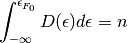
in which  is the Fermi energy at zero temperature for the
non-interacting system such that
is the Fermi energy at zero temperature for the
non-interacting system such that
(15)
This procedure of defining a zero temperature
non-interacting Fermi energy( and thus
  ) allows to keep the particle
population fixed when correlations are included into the
problem [Yu2011] [Florens2004].
) allows to keep the particle
population fixed when correlations are included into the
problem [Yu2011] [Florens2004].
Introducing doping
The previous introduction to the slave spins treats the Hubbard Hamiltonian
and deals with the quartic term that deals with the correlations. But it is
only valid in the simplified case of degenerate orbitals at
half-filling. When aiming to introduce doping, a more elaborate formulation is
required. The fact is that the Spin Hamiltonian is unable to manage doping
cases as previously formulated, since it is always populated by 2 spin which
flip by the action of the operator  in a balanced manner. This is
equivalent to the real electron hopping from one lattice site to the next.
in a balanced manner. This is
equivalent to the real electron hopping from one lattice site to the next.
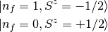
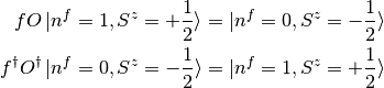
In the case of electron or hole doping, the fermion Hamiltonian deals with it through the chemical potential, which doesn’t appear in the Spin Hamiltonian. Then a new generic Spin operator needs to be introduced, to treat this spin flip unbalance in the Spin system and deal with the doping cases. It is an mixture of the spin raising and lowering operators.
(16)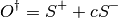
The inclusion of the gauge parameter  originates from the study of the
action of the real creation and annihilation operators
originates from the study of the
action of the real creation and annihilation operators  into
the
real states. And then how the new operators act into the extended Hilbert
space. The reference case is such
into
the
real states. And then how the new operators act into the extended Hilbert
space. The reference case is such
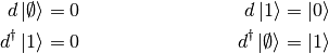
The first conditions on the left can be assured by the fermion operator.
the  operator does not play any role. For second set of conditions
only three out of four matrix elements of the operator can be determined,
which implies that
(17)
Which is in correspondence with the previous formulation of equation
(16). can be an arbitrary complex number and it is tuned
in order to give rise to the most physical approximation scheme, by imposing
that it correctly reproduces solvable limits of the problem such as the
non-interacting limit.
The non-interacting limit
Starting with a Tight Binding Hamiltonian that only includes the kinetic energy term and a contribution from the chemical potential to control the doping, the new operators are introduced. Treating a single orbital case of atoms in a lattice.
Here the Lagrange multiplier is treated as individual to every site. Using first a Hartree-Fock approximation in the tight binding term and respecting the restriction set by the Lagrange multiplier, it is possible to separate the Hamiltonian into 2 coupled effective ones.
The parameters  hopping renormalization factor,
  slave-spin
exchange constant and
slave-spin
exchange constant and  in these expressions are determined from the
coupled self-consistency equations:
in these expressions are determined from the
coupled self-consistency equations:
(18)
(19)
(20)
One further approximation needs to be applied, and it is to treat the spin Hamiltonian within a Weiss mean field, in which a single site is embedded in an effective field of its surroundings. The spin Hamiltonian becomes:
Where the mean field 
Choosing the gauge c
The condition set, to reproduce the non-interacting case is  ,
where the quasiparticle residum
,
where the quasiparticle residum  . In the single
site approximation
. In the single
site approximation  by construction, and only it’s unitary value
remains to be enforced . The non-interacting spin Hamiltonian is treated
suppressing the spin index
by construction, and only it’s unitary value
remains to be enforced . The non-interacting spin Hamiltonian is treated
suppressing the spin index  since in this case up-spin and down-spin
fermions are decoupled.
since in this case up-spin and down-spin
fermions are decoupled.
It is possible to diagonalize the Hamiltonian for one slave spin in the  basis. The ground state eigenvalue
  and the corresponding
eigenstate are.
and the corresponding
eigenstate are.
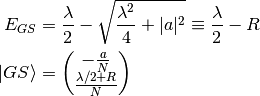
Where 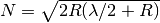 and
and  . The expected
values of
. The expected
values of  and are:
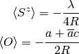
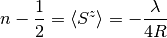
It is clearly seen that the Lagrange multiplier depends on the
density  and it is adjusted to satisfy the constraint equation:
(21)
and needs to be tuned to match the condition
(22)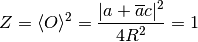
It is possible to eliminate from the conditions by squaring
(21) and using the relation (22), following the next derivation:
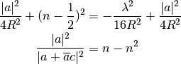
Then it is possible to choose real, making also  and
and  real. The
expression for is found to be independent of the mean field :
real. The
expression for is found to be independent of the mean field :
Hund’s coupling
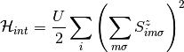
The interaction Hamiltonian in this multiorbital systems then becomes:
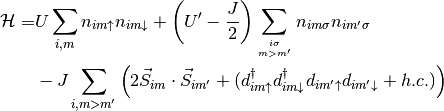
Where  is the intra orbital Hubbard interaction and
  is the
interorbital interaction
is the
interorbital interaction  is the total spin in an orbital.
Which is then traded into slave spin variables to give:
is the total spin in an orbital.
Which is then traded into slave spin variables to give: